Exploration of the chemical space using RDKIT and cheminformatics

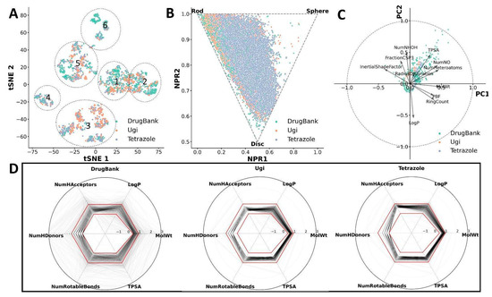
In this workflow, I decided to demonstrate how I conducted the analysis for my recent publication: In Silico Design and Selection of New Tetrahydroisoquinoline-Based CD44 Antagonist Candidates [https://doi.org/10.3390/molecules26071877].

As I mentioned in the previous post, I will not go into detail about the analysis of their usage, but rather the code implementation. I believe you can find better explanations of methods and their applications in literature (e.g., my paper!!).

I decided to make this workflow interactive so that the explanation and chemical space exploration would be clearer.

Importing the libraries

'''
Plotting libraries
'''
import pandas as pd
import matplotlib.cm as cm
from matplotlib import pyplot as plt
import seaborn as sns
import numpy as np

'''
What we'll need for analysis, clustering, etc.
'''
from sklearn.decomposition import PCA
from sklearn.preprocessing import StandardScaler
from sklearn.metrics import silhouette_samples, silhouette_score
from sklearn.cluster import KMeans
from sklearn import datasets, decomposition
from sklearn.manifold import TSNE

'''
Of course the powerful RDKIT for cheminformatics <3
'''
from rdkit import Chem, DataStructs
from rdkit.Chem import AllChem, MACCSkeys, Descriptors, Descriptors3D, Draw, rdMolDescriptors, Draw, PandasTools
from rdkit.DataManip.Metric.rdMetricMatrixCalc import GetTanimotoSimMat, GetTanimotoDistMat
from rdkit.Chem.Draw import IPythonConsole

'''
Some utilities
'''
import progressbar
from math import pi

%config Completer.use_jedi = False
PandasTools.RenderImagesInAllDataFrames(images=True)

For this workflow I’ll use FDA apporved molecules taken from ZINC15 [https://zinc15.docking.org/catalogs/dbfda/substances/subsets/world/]

If your file format is Mol2, maybe you can need my Mol2MolSupplier for RDKIT. [https://chem-workflows.com/articles/2020/03/23/building-a-multi-molecule-mol2-reader-for-rdkit-v2/]

mols=Chem.SDMolSupplier('FDA_approved.sdf')
print (len(mols)) #To check how many molecules there are in the file

1615

Despite the fact that not all of the descriptors in the cell below are required, I decided to include them to demonstrate the large number of descriptors that RDKIT can compute (2D and 3D).

bar=progressbar.ProgressBar(max_value=len(mols))
table=pd.DataFrame()
for i,mol in enumerate(mols):
    Chem.SanitizeMol(mol)
    table.loc[i,'smiles']=Chem.MolToSmiles(mol)
    table.loc[i,'Mol']=mol
    table.loc[i,'MolWt']=Descriptors.MolWt(mol)
    table.loc[i,'LogP']=Descriptors.MolLogP(mol)
    table.loc[i,'NumHAcceptors']=Descriptors.NumHAcceptors(mol)
    table.loc[i,'NumHDonors']=Descriptors.NumHDonors(mol)
    table.loc[i,'NumHeteroatoms']=Descriptors.NumHeteroatoms(mol)
    table.loc[i,'NumRotatableBonds']=Descriptors.NumRotatableBonds(mol)
    table.loc[i,'NumHeavyAtoms']=Descriptors.HeavyAtomCount (mol)
    table.loc[i,'NumAliphaticCarbocycles']=Descriptors.NumAliphaticCarbocycles(mol)
    table.loc[i,'NumAliphaticHeterocycles']=Descriptors.NumAliphaticHeterocycles(mol)
    table.loc[i,'NumAliphaticRings']=Descriptors.NumAliphaticRings(mol)
    table.loc[i,'NumAromaticCarbocycles']=Descriptors.NumAromaticCarbocycles(mol)
    table.loc[i,'NumAromaticHeterocycles']=Descriptors.NumAromaticHeterocycles(mol)
    table.loc[i,'NumAromaticRings']=Descriptors.NumAromaticRings(mol)
    table.loc[i,'RingCount']=Descriptors.RingCount(mol)
    table.loc[i,'FractionCSP3']=Descriptors.FractionCSP3(mol)

    table.loc[i,'TPSA']=Descriptors.TPSA(mol)
    table.loc[i,'NPR1']=rdMolDescriptors.CalcNPR1(mol)
    table.loc[i,'NPR2']=rdMolDescriptors.CalcNPR2(mol)
    table.loc[i,'InertialShapeFactor']=Descriptors3D.InertialShapeFactor(mol)
    table.loc[i,'RadiusOfGyration']=Descriptors3D.RadiusOfGyration(mol)
    bar.update(i+1)

 25% (405 of 1615) |#####                | Elapsed Time: 0:00:02 ETA:   0:00:07RDKit WARNING: [17:47:08] Warning: molecule is tagged as 3D, but all Z coords are zero
 64% (1038 of 1615) |############        | Elapsed Time: 0:00:06 ETA:   0:00:04RDKit WARNING: [17:47:12] Warning: molecule is tagged as 3D, but all Z coords are zero
 72% (1163 of 1615) |##############      | Elapsed Time: 0:00:07 ETA:   0:00:03RDKit WARNING: [17:47:13] Warning: molecule is tagged as 3D, but all Z coords are zero
 82% (1339 of 1615) |################    | Elapsed Time: 0:00:09 ETA:   0:00:02RDKit WARNING: [17:47:14] Warning: molecule is tagged as 3D, but all Z coords are zero
 86% (1399 of 1615) |#################   | Elapsed Time: 0:00:09 ETA:   0:00:01RDKit WARNING: [17:47:15] Warning: molecule is tagged as 3D, but all Z coords are zero
100% (1615 of 1615) |####################| Elapsed Time: 0:00:11 ETA:  00:00:00

table.head(5) #Let's take a look to the table

	smiles	Mol	MolWt	LogP	NumHAcceptors	NumHDonors	NumHeteroatoms	NumRotatableBonds	NumHeavyAtoms	NumAliphaticCarbocycles	...	NumAromaticCarbocycles	NumAromaticHeterocycles	NumAromaticRings	RingCount	FractionCSP3	TPSA	NPR1	NPR2	InertialShapeFactor	RadiusOfGyration
0	CC(=O)Oc1ccccc1C(=O)O		180.159	1.3101	3.0	1.0	4.0	2.0	13.0	0.0	...	1.0	0.0	1.0	1.0	0.111111	63.60	0.457886	0.674973	0.001616	2.377590
1	NCC(CC(=O)O)c1ccc(Cl)cc1		213.664	1.8570	2.0	2.0	4.0	4.0	14.0	0.0	...	1.0	0.0	1.0	1.0	0.300000	63.32	0.333958	0.800705	0.001482	2.927355
2	CC(C[N+](C)(C)C)OC(N)=O		161.225	0.1764	2.0	1.0	4.0	3.0	11.0	0.0	...	0.0	0.0	0.0	0.0	0.857143	52.32	0.203294	0.946857	0.005081	2.615321
3	CN(C)CCC(c1ccc(Br)cc1)c1ccccn1		319.246	3.9277	2.0	0.0	3.0	5.0	19.0	0.0	...	1.0	1.0	2.0	2.0	0.312500	16.13	0.233137	0.837523	0.000799	3.938401
4	CN(C)CCOC(c1ccc(Cl)cc1)c1ccccn1		290.794	3.4026	3.0	0.0	4.0	6.0	20.0	0.0	...	1.0	1.0	2.0	2.0	0.312500	25.36	0.521272	0.564122	0.000295	3.753247

5 rows × 22 columns

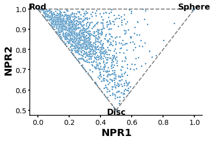
Normalized Principal Moment of Inertia ratios (NPR) plot to describe molecules shapes

plt.rcParams['axes.linewidth'] = 1.5
plt.figure(figsize=(6,4))

ax=sns.scatterplot(x='NPR1',y='NPR2',data=table,s=10,linewidth=0.5,alpha=1)
x1, y1 = [0.5, 0], [0.5, 1]
x2, y2 = [0.5, 1], [0.5, 1]
x3, y3 = [0,1],[1,1]

plt.plot(x1, y1,x2,y2,x3,y3,c='gray',ls='--',lw=2)

plt.xlabel ('NPR1',fontsize=20,fontweight='bold')

plt.ylabel ('NPR2',fontsize=20,fontweight='bold')

ax.spines['top'].set_visible(False)
ax.spines['right'].set_visible(False)

plt.text(0, 1.01,s='Rod',fontsize=16,horizontalalignment='center',verticalalignment='center',fontweight='bold')
plt.text(1, 1.01,s='Sphere',fontsize=16,horizontalalignment='center',verticalalignment='center',fontweight='bold')
plt.text(0.5, 0.49,s='Disc',fontsize=16,horizontalalignment='center',verticalalignment='center',fontweight='bold')

plt.tick_params ('both',width=2,labelsize=14)
plt.tight_layout()

plt.show()

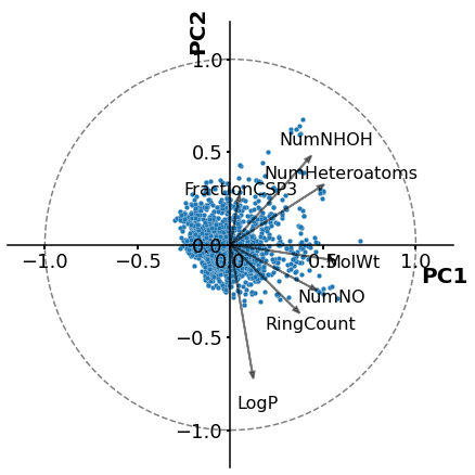
Principal Component Analysis (PCA)

The molecules are described by their phisicpochemycal terms

More information about the coding and implementation of this method can be found in my previous post [https://chem-workflows.com/articles/2019/07/02/exploring-the-chemical-space-by-pca/].

I won’t go into detail about the following models or the descriptors used to perform the analysis. More information on method validations can be found in my paper and supplementary materials [https://www.mdpi.com/1420-3049/26/7/1877].

descriptors = table[['MolWt', 'LogP','NumHeteroatoms','RingCount','FractionCSP3', 'TPSA','RadiusOfGyration']].values #The non-redundant molecular descriptors chosen for PCA
descriptors_std = StandardScaler().fit_transform(descriptors) #Important to avoid scaling problems between our different descriptors
pca = PCA()
descriptors_2d = pca.fit_transform(descriptors_std)
descriptors_pca= pd.DataFrame(descriptors_2d) # Saving PCA values to a new table
descriptors_pca.index = table.index
descriptors_pca.columns = ['PC{}'.format(i+1) for i in descriptors_pca.columns]
descriptors_pca.head(5) #Displays the PCA table

	PC1	PC2	PC3	PC4	PC5	PC6	PC7
0	-2.030216	0.330955	-1.476264	0.206369	-0.179943	-0.161048	0.035943
1	-1.691955	0.238768	-0.666979	0.385343	-0.158692	-0.165407	0.060639
2	-2.230606	1.424068	1.347416	0.325014	-0.186890	0.154174	0.032474
3	-1.199580	-1.225828	-0.227412	0.479184	-0.078112	0.058030	-0.369111
4	-1.184750	-0.878367	-0.346455	0.366559	-0.059148	0.179514	-0.211592

print(pca.explained_variance_ratio_) #Let's plot PC1 vs PC2
print(sum(pca.explained_variance_ratio_))

[0.4693332  0.260776   0.138159   0.08058236 0.02983395 0.01176394
 0.00955153]
1.0

# This normalization will be performed just for PC1 and PC2, but can be done for all the components.
#The normalization is to plot PCA values in 0-1 sacle and include the vectors (features to the plot)

scale1 = 1.0/(max(descriptors_pca['PC1']) - min(descriptors_pca['PC1']))
scale2 = 1.0/(max(descriptors_pca['PC2']) - min(descriptors_pca['PC2']))

# And we add the new values to our PCA table
descriptors_pca['PC1_normalized']=[i*scale1 for i in descriptors_pca['PC1']]
descriptors_pca['PC2_normalized']=[i*scale2 for i in descriptors_pca['PC2']]

descriptors_pca.head(5) # The PCA table now has the normalized PC1 and PC2

	PC1	PC2	PC3	PC4	PC5	PC6	PC7	PC1_normalized	PC2_normalized
0	-2.030216	0.330955	-1.476264	0.206369	-0.179943	-0.161048	0.035943	-0.171975	0.033625
1	-1.691955	0.238768	-0.666979	0.385343	-0.158692	-0.165407	0.060639	-0.143322	0.024259
2	-2.230606	1.424068	1.347416	0.325014	-0.186890	0.154174	0.032474	-0.188949	0.144685
3	-1.199580	-1.225828	-0.227412	0.479184	-0.078112	0.058030	-0.369111	-0.101614	-0.124544
4	-1.184750	-0.878367	-0.346455	0.366559	-0.059148	0.179514	-0.211592	-0.100357	-0.089242

plt.rcParams['axes.linewidth'] = 1.5
plt.figure(figsize=(6,6))

ax=sns.scatterplot(x='PC1_normalized',y='PC2_normalized',data=descriptors_pca,s=20,palette=sns.color_palette("Set2", 3),linewidth=0.2,alpha=1)

plt.xlabel ('PC1',fontsize=20,fontweight='bold')
ax.xaxis.set_label_coords(0.98, 0.45)
plt.ylabel ('PC2',fontsize=20,fontweight='bold')
ax.yaxis.set_label_coords(0.45, 0.98)

ax.spines['left'].set_position(('data', 0))
ax.spines['bottom'].set_position(('data', 0))
ax.spines['top'].set_visible(False)
ax.spines['right'].set_visible(False)


lab=['MolWt', 'LogP','NumHeteroatoms','RingCount','FractionCSP3',
     'NumNHOH', 'NumNO', 'TPSA','PBF',
     'InertialShapeFactor','RadiusOfGyration'] #Feature labels

l=np.transpose(pca.components_[0:2, :]) ## We will get the components eigenvectors (main features) for PC1 and PC2

n = l.shape[0]
for i in range(n):
    plt.arrow(0, 0, l[i,0], l[i,1],color= 'k',alpha=0.5,linewidth=1.8,head_width=0.025)
    plt.text(l[i,0]*1.25, l[i,1]*1.25, lab[i], color = 'k',va = 'center', ha = 'center',fontsize=16)

circle = plt.Circle((0,0), 1, color='gray', fill=False,clip_on=True,linewidth=1.5,linestyle='--')

plt.tick_params ('both',width=2,labelsize=18)

ax.add_artist(circle)
plt.xlim(-1.2,1.2)
plt.ylim(-1.2,1.2)
plt.tight_layout()
plt.show()

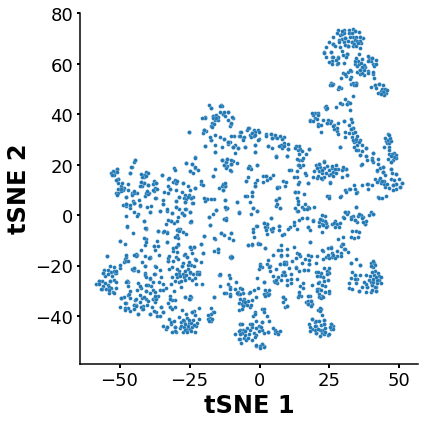
t-SNE (T-distributed Stochastic Neighbor Embedding)

Molecules are described by their strcutural features

Unlike PCA, in t-SNE analysis, we compare molecues based on their structural features (fingerprints, MACCSKeys, …) not physicochemical properties.

smiles = list(table["smiles"])
smi=[Chem.MolFromSmiles(x) for x in smiles]
fps =  [MACCSkeys.GenMACCSKeys(x) for x in smi] # In this example I'll use MACCSKeys
tanimoto_sim_mat_lower_triangle=GetTanimotoSimMat(fps) #This compute a similartity matrix between all the molecules
n_mol = len(fps)
similarity_matrix = np.ones([n_mol,n_mol])
i_lower= np.tril_indices(n=n_mol,m=n_mol,k=-1)
i_upper= np.triu_indices(n=n_mol,m=n_mol,k=1)
similarity_matrix[i_lower] = tanimoto_sim_mat_lower_triangle
similarity_matrix[i_upper] = similarity_matrix.T[i_upper]
distance_matrix = np.subtract(1,similarity_matrix) #This is the similarity matrix of all vs all molecules in our table

TSNE_sim = TSNE(n_components=2,init='pca',random_state=90, angle = 0.3,perplexity=50).fit_transform(distance_matrix) #Remember to always tune the parameters acording your dataset!!
tsne_result = pd.DataFrame(data = TSNE_sim , columns=["TC1","TC2"]) # New table containing the tSNE results
tsne_result.head(5) #A new table containing the tSNE results

	TC1	TC2
0	33.624451	28.951748
1	22.952942	21.361393
2	13.488312	1.682003
3	26.264500	-43.811687
4	-24.879755	1.109156

plt.rcParams['axes.linewidth'] = 1.5
fig, ax = plt.subplots(figsize=(6,6))

ax=sns.scatterplot(x='TC1',y='TC2',data=tsne_result,s=15,linewidth=0.2,alpha=1)


plt.xlabel ('tSNE 1',fontsize=24,fontweight='bold')

plt.ylabel ('tSNE 2',fontsize=24,fontweight='bold')

plt.tick_params ('both',width=2,labelsize=18)

ax.spines['top'].set_visible(False)
ax.spines['right'].set_visible(False)
handles, labels = ax.get_legend_handles_labels()

#ax.legend(handles=handles[1:], labels=labels[1:])

#plt.legend(loc='lower right',frameon=False,prop={'size': 22},ncol=1)

plt.tight_layout()
plt.show()

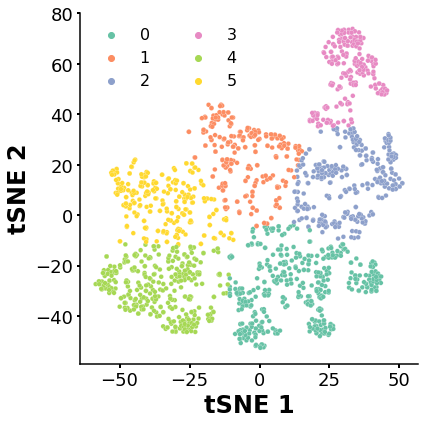
K-means clustering

Identify clusters of molecues with similar features (structure) after t-SNE

range_n_clusters = [2, 3, 4, 5, 6, 7, 8, 9, 10] # To explore the "best" number of cluster to clasify our molecules
for n_clusters in range_n_clusters:
    kmeans = KMeans(n_clusters=n_clusters, random_state=10)
    cluster_labels = kmeans.fit_predict(tsne_result[['TC1','TC2']])
    silhouette_avg = silhouette_score(tsne_result[['TC1','TC1']], cluster_labels)
    print("For n_clusters =", n_clusters,
          "The average silhouette_score is :", silhouette_avg) #This will print the silhouette score, as higher as our data is better distributed inside the clusters

For n_clusters = 2 The average silhouette_score is : 0.36085638
For n_clusters = 3 The average silhouette_score is : 0.2601781
For n_clusters = 4 The average silhouette_score is : 0.11969557
For n_clusters = 5 The average silhouette_score is : 0.0039482377
For n_clusters = 6 The average silhouette_score is : -0.04504208
For n_clusters = 7 The average silhouette_score is : -0.062240764
For n_clusters = 8 The average silhouette_score is : -0.052293032
For n_clusters = 9 The average silhouette_score is : -0.04769651
For n_clusters = 10 The average silhouette_score is : -0.04771827

WARNING

Despite the fact that the silhouette calculations yielded very poor results in classifying the molecules, I’ll cluster the dataset into six clusters for demonstration purposes.

kmeans = KMeans(n_clusters=6, random_state=10) # We define the best number of clusters (6)
clusters = kmeans.fit(tsne_result[['TC1','TC2']]) #TC1vs TC2

tsne_result['Cluster'] = pd.Series(clusters.labels_, index=tsne_result.index)
tsne_result.head(5) #The tSNE table now contains the numer of cluster for each element

	TC1	TC2	Cluster
0	33.624451	28.951748	2
1	22.952942	21.361393	2
2	13.488312	1.682003	2
3	26.264500	-43.811687	0
4	-24.879755	1.109156	5

plt.rcParams['axes.linewidth'] = 1.5
fig, ax = plt.subplots(figsize=(6,6))

ax=sns.scatterplot(x='TC1',y='TC2',data=tsne_result, hue='Cluster',s=22,palette=sns.color_palette("Set2", 6),linewidth=0.2,alpha=1)


plt.xlabel ('tSNE 1',fontsize=24,fontweight='bold')

plt.ylabel ('tSNE 2',fontsize=24,fontweight='bold')

plt.tick_params ('both',width=2,labelsize=18)

ax.spines['top'].set_visible(False)
ax.spines['right'].set_visible(False)

handles, labels = ax.get_legend_handles_labels()

ax.legend(handles=handles[1:], labels=labels[1:])

plt.legend(loc='best',frameon=False,prop={'size': 16},ncol=2)

plt.tight_layout()
plt.show()

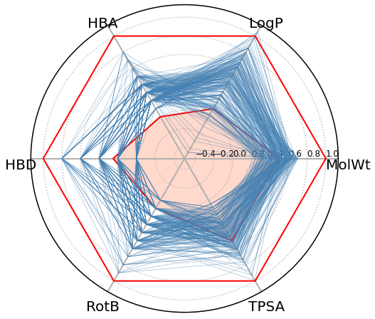
Radar chart of Beyond Lipinski’s Rule of Five (bRo5)

This plot can provide information about a compound’s ability to be administered orally.

data=pd.DataFrame() # I'll create a new table containing the normalized bRo5 values of our compounds

data['MolWt']=[i/500 for i in table['MolWt']]
data['LogP']=[i/5 for i in table['LogP']]
data['HBA']=[i/10 for i in table['NumHAcceptors']]
data['HBD']=[i/5 for i in table['NumHDonors']]
data['RotB']=[i/10 for i in table['NumRotatableBonds']]
data['TPSA']=[i/140 for i in table['TPSA']]

categories=list(data.columns)  # This will set up the parameters for the angles of the radar plot.
N = len(categories)
values=data[categories].values[0]
values=np.append(values,values[:1])
angles = [n / float(N) * 2 * pi for n in range(N)]
angles += angles[:1]

Ro5_up=[1,1,1,1,1,1,1] #The upper limit for bRo5
Ro5_low=[0.5,0.1,0,0.25,0.1,0.5,0.5]  #The lower limit for bRo5

fig=plt.figure(figsize=(6,6))

ax = fig.add_axes([1, 1, 1, 1],projection='polar')

plt.xticks(angles[:-1], categories,color='k',size=20,ha='center',va='top',fontweight='book')

plt.tick_params(axis='y',width=4,labelsize=12, grid_alpha=0.05)

ax.set_rlabel_position(0)

ax.plot(angles, Ro5_up, linewidth=2, linestyle='-',color='red')
ax.plot(angles, Ro5_low, linewidth=2, linestyle='-',color='red')

#ax.fill(angles, Ro5_up, 'red', alpha=0.2)
ax.fill(angles, Ro5_low, 'orangered', alpha=0.2)

for i in data.index[:250]: #I'll just show the profile for the first 250 molecules in the table for clarity of the plot
    values=data[categories].values[i]
    values=np.append(values,values[:1])
    ax.plot(angles, values, linewidth=0.7 ,color='steelblue',alpha=0.5)
    #ax.fill(angles, values, 'C2', alpha=0.025)

ax.grid(axis='y',linewidth=1.5,linestyle='dotted',alpha=0.8)
ax.grid(axis='x',linewidth=2,linestyle='-',alpha=1)

plt.show()

Remarks

I hope this workflow is useful to you. Please do not be hesitant to thoroughly examine the foundation and methods when you’re implementing any of this analysis.

Have a great time!!!