Similarity analysis of compound databases

In this chem-workflow, I will show you a strategy to calculate the similarity of a molecule database in a straightforward manner.

For this purpose, I will use a fraction of the REAL Compound Library of Enamine. You can read more about the database here.

Despite I will use a SMILES file, this analysis can be performed from SDF codes of molecules or any other format in the same way. Just be sure of using the appropriate supplier for loading your molecules into RDKIT.

Importing the libraries we need

import os
import pandas as pd
import numpy as np
import matplotlib.pyplot as plt
from matplotlib import gridspec

from rdkit import Chem, DataStructs
from rdkit.Chem.Fingerprints import FingerprintMols
from rdkit.Chem import Draw

# All we need for clustering
from scipy.cluster.hierarchy import dendrogram, linkage

Loading and visualizing the molecules

The library contains more than 8 000 000 SMILES codes (size 542.8 M). But we can read the .smiles file as a text file to keep the fist 100 molecules.

# The result of this code will be:
working_library=[]
with open('Enamine_REAL_diversity.smiles','r') as file:
    for index,line in enumerate(file):
        if 0<index<=1: # Kee the fist smile code as example
            print (index, line.split())

1 ['CC(C)C(C)(C)SCC=CBr', 'PV-002312932038']

The result of the above cell is a list which first element (0) is the SMILES codes of the molecule, and the second element (1), the name.

So, we can use the same code to convert SMILES codes to RDKIT molecules.

working_library=[]
with open('Enamine_REAL_diversity.smiles','r') as file:
    for index,line in enumerate(file):
        if 0<index<=100: # Molecules we want (0 is omitted because the fist line (0) of file is the header, not SMILES code)
            mol=Chem.MolFromSmiles(line.split()[0]) # Converting SMILES codes into rdkit mol
            mol.SetProp('_Name',line.split()[1]) # Adding the name for each molecule
            working_library.append(mol)

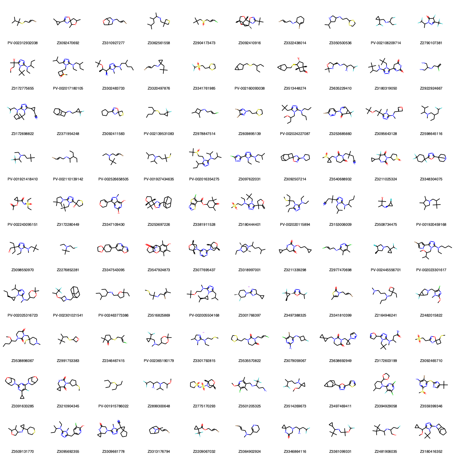
Now we have a list of 100 RDKIT type molecules to perform our similarity analysis.

Let´s draw them to see what is inside.

Draw.MolsToGridImage(working_library,molsPerRow=10,subImgSize=(150,150),legends=[mol.GetProp('_Name') for mol in working_library])

Getting the fingerprints for comparison

For fingerprint similarity analysis, we first need to get the fingerprints for each molecule.

For such purpose we type:

fps= [FingerprintMols.FingerprintMol(mol) for mol in working_library]

As result we have n fingerprints as n molecules:

print(len(working_library))
print(len(fps))

100
100

And we can get the similarity for each pair of molecules.

For instance mol_1 as reference and mol_2 as target.

DataStructs.FingerprintSimilarity(fps[0],fps[1])

0.3438735177865613

Following the above example, we can construct all vs all analysis to see the similarity within our database (Something similar can be found in another Chem-workflow of this site -click here to see that entry-)

size=len(working_library)
hmap=np.empty(shape=(size,size))
table=pd.DataFrame()
for index, i in enumerate(fps):
    for jndex, j in enumerate(fps):
        similarity=DataStructs.FingerprintSimilarity(i,j)
        hmap[index,jndex]=similarity
        table.loc[working_library[index].GetProp('_Name'),working_library[jndex].GetProp('_Name')]=similarity

Let´s take a look to the similarity values

table.head(10) # just the first 10 values due to our table in 100 x 100

	PV-002312932038	Z3092470692	Z3310927277	Z3362561558	Z2904173473	Z3092410916	Z3322438014	Z3350500536	PV-002106209714	Z2790107381	...	Z3509131770	Z3095692355	Z3309661778	Z3313176794	Z2209067032	Z3364902924	Z3346864116	Z3361099331	Z2481906035	Z3180416352
PV-002312932038	1.000000	0.343874	0.342995	0.339394	0.379845	0.342520	0.369792	0.319588	0.282353	0.331984	...	0.324675	0.335938	0.339844	0.324324	0.317308	0.333333	0.294931	0.312821	0.303922	0.335938
Z3092470692	0.343874	1.000000	0.512712	0.307036	0.349020	0.635063	0.428270	0.411765	0.505882	0.395076	...	0.413333	0.257565	0.346515	0.377399	0.453975	0.356688	0.291557	0.410638	0.434599	0.350902
Z3310927277	0.342995	0.512712	1.000000	0.313480	0.362319	0.510204	0.349162	0.369628	0.497674	0.445676	...	0.528947	0.474227	0.494071	0.430380	0.361413	0.369231	0.392105	0.416918	0.380682	0.485030
Z3362561558	0.339394	0.307036	0.313480	1.000000	0.315789	0.317526	0.326389	0.508000	0.456044	0.308789	...	0.371429	0.306383	0.315261	0.409639	0.253918	0.278810	0.300912	0.420849	0.458333	0.309572
Z2904173473	0.379845	0.349020	0.362319	0.315789	1.000000	0.358268	0.335000	0.306533	0.275862	0.348178	...	0.365639	0.351562	0.355469	0.276923	0.305164	0.276596	0.289593	0.306533	0.330049	0.351562
Z3092410916	0.342520	0.635063	0.510204	0.317526	0.358268	1.000000	0.431772	0.424490	0.503906	0.427624	...	0.411908	0.283253	0.384665	0.382716	0.447791	0.362705	0.291517	0.417695	0.446721	0.408696
Z3322438014	0.369792	0.428270	0.349162	0.326389	0.335000	0.431772	1.000000	0.344512	0.454976	0.372768	...	0.360000	0.418410	0.432271	0.421233	0.307042	0.397260	0.344262	0.333333	0.340299	0.414000
Z3350500536	0.319588	0.411765	0.369628	0.508000	0.306533	0.424490	0.344512	1.000000	0.456311	0.389522	...	0.452830	0.419831	0.430862	0.423611	0.307692	0.300000	0.428152	0.418605	0.423077	0.426829
PV-002106209714	0.282353	0.505882	0.497674	0.456044	0.275862	0.503906	0.454976	0.456311	1.000000	0.504032	...	0.508621	0.513725	0.511719	0.423645	0.514286	0.414141	0.490826	0.538462	0.557789	0.513725
Z2790107381	0.331984	0.395076	0.445676	0.308789	0.348178	0.427624	0.372768	0.389522	0.504032	1.000000	...	0.326648	0.424028	0.465536	0.342529	0.455172	0.360849	0.294028	0.356659	0.410959	0.444564

10 rows × 100 columns

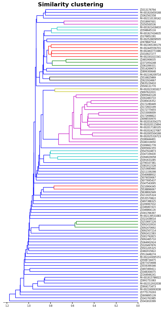
We can cluster our compound by similarity applying a linkage hierarchical clustering (HCL) analysis (Something similar can be found in another Chem-workflow of this site -click here to see that entry-).

I won´t discuss the different methods for HCL (e.g. single, complete, average, etc). Because literature is plenty of such discussions, for example, you can check the skit-learn documentation.

HCL clustering

linked = linkage(hmap,'single')
labelList = [mol.GetProp('_Name') for mol in working_library]

plt.figure(figsize=(8,15))

ax1=plt.subplot()
o=dendrogram(linked,
            orientation='left',
            labels=labelList,
            distance_sort='descending',
            show_leaf_counts=True)

ax1.spines['left'].set_visible(False)
ax1.spines['top'].set_visible(False)
ax1.spines['right'].set_visible(False)
plt.title('Similarity clustering',fontsize=20,weight='bold')
plt.tick_params ('both',width=2,labelsize=8)
plt.tight_layout()
plt.show()

Now let´s sort our initial values by the HCL analysis.

# This will give us the clusters in order as the last plot
new_data=list(reversed(o['ivl']))

# we create a new table with the order of HCL
hmap_2=np.empty(shape=(size,size))
for index,i in enumerate(new_data):
    for jndex,j in enumerate(new_data):
        hmap_2[index,jndex]=table.loc[i].at[j]

figure= plt.figure(figsize=(30,30))
gs1 = gridspec.GridSpec(2,7)
gs1.update(wspace=0.01)
ax1 = plt.subplot(gs1[0:-1, :2])
dendrogram(linked, orientation='left', distance_sort='descending',show_leaf_counts=True,no_labels=True)
ax1.spines['left'].set_visible(False)
ax1.spines['top'].set_visible(False)
ax1.spines['right'].set_visible(False)

ax2 = plt.subplot(gs1[0:-1,2:6])
f=ax2.imshow (hmap_2, cmap='PRGn_r', interpolation='nearest')

ax2.set_title('Fingerprint Similarity',fontsize=20,weight='bold')
ax2.set_xticks (range(len(new_data)))
ax2.set_yticks (range(len(new_data)))
ax2.set_xticklabels (new_data,rotation=90,size=8)
ax2.set_yticklabels (new_data,size=8)

ax3 = plt.subplot(gs1[0:-1,6:7])
m=plt.colorbar(f,cax=ax3,shrink=0.75,orientation='vertical',spacing='uniform',pad=0.01)
m.set_label ('Fingerprint Similarity')

plt.tick_params ('both',width=2)
plt.plot()

[]

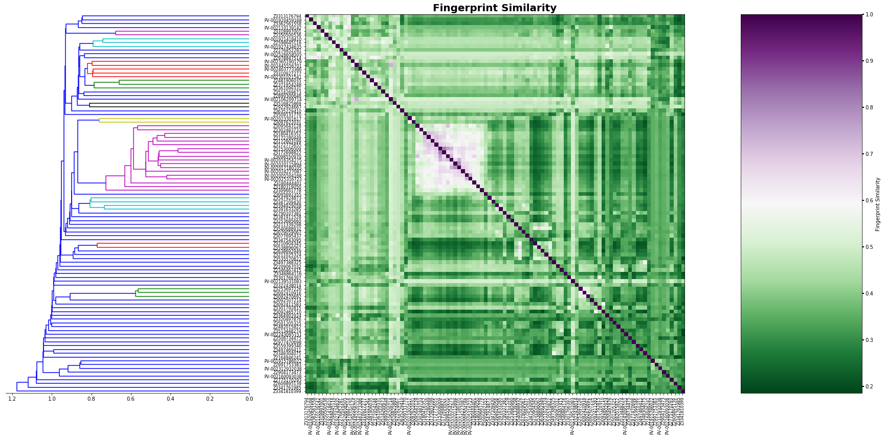
As you can see, our approach was able to identify several clusters based on fingerprint similarity, however. RDKIT can also calculate frequent-used similarity models. For example Tanimoto, Dice, Cosine, Sokal, Russel, Kulczynski, McConnaughey, and Tversky. The implementation is very easy and can be set by doing:

similarity=DataStructs.FingerprintSimilarity(i,j, metric=DataStructs.DiceSimilarity)

where:

metric - Should be one of the different methods described above.