Brief introduction to Molecular Dynamics analysis with MDanalysis
![]()
In this entry, I’d like to present a basic analysis of molecular dynamics (MD) systems using MD Analysis (MDA).
Despite its simplicity, this workflow could be a good starting point for those interested in MD analysis with Python and Jupyter notebooks.
Importing the libraries
[1]:
'''
Main modules for this workflow
'''
import MDAnalysis as mda
from MDAnalysis.analysis import align, rms
from MDAnalysis.tests.datafiles import PSF, DCD #These are testing files from MDanalysis, when using your own MD files don't need to import this anymore

'''
Packages to visualize, plot data, and utilities
'''

import pandas as pd
import matplotlib as mpl
from matplotlib import pyplot as plt
import seaborn as sns
import py3Dmol
import progressbar # Not needed but useful to see analysis progress


%matplotlib inline
%config Completer.use_jedi = False
[2]:
'''
MDA version
'''

mda.__version__
[2]:
'0.20.1'
MDA loads MD systems as “Universe,” which contains all trajectory and topology data. Keep in mind that MDA accepts a wide range of MD formats (gromacs, amber, NAMD, …).
[3]:
u=mda.Universe(PSF,DCD) #Loading the MD data topology=PSF, trajectory=DCD;
print(u.segments,'with {} residues'.format(len(u.residues))) #Inspecting our system
<SegmentGroup [<Segment 4AKE>]> with 214 residues
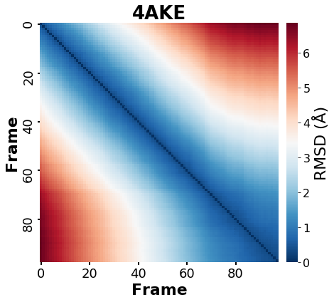
Conducting a Pairwise RMSD analysis on the MD simulation
The pairwise analysis is a method for observing a molecule’s RMSD changes over simulation time in order to identify related conformations (or states).
A pairwise analysis in MDA is simple to perform by aligning and computing the RMSD over the simulation time.
Depending on the interest shown by the user. The RMSD can be calculated for various system selections. Protein, ligand, protein-ligand complex, a list of residues, only one chain, and so on.
MDA allows for a robust and well-documented selection algebra in: https://docs.mdanalysis.org/stable/documentation_pages/selections.html
For this example, I’ll run a pairwise RMSD on the entire “Universe”, which is made up of only the ADENYLATE KINASE protein (PDB: 4AKE) and no other organic molecules or solven. As a result, the pairwise RMSD must be consistent with the protein analysis.
[4]:
bar=progressbar.ProgressBar(max_value=len(u.trajectory)) #loading a progressbar using the lenght of the simulation
RMSD_hmap=pd.DataFrame() # The Pairwise values will be saved on a pandas dataFrame
for i in range(len(u.trajectory)): #Depending on simulation 's lenght the calculations could be time-consuming. It could be advisable to compute the RMSD in a different step interval than 1
    for j in range(len(u.trajectory)):
        bb = u.select_atoms('backbone') # I'll compute only Backbone RMSD of the protein
        u.trajectory[i]
        A = bb.positions.copy() # coordinates of first frame
        u.trajectory[j]         # forward to second frame
        B = bb.positions.copy()  # coordinates of second frame
        rmsd=rms.rmsd(A, B, center=True, superposition=True) # Center and superposition is enabled to consider only protein movements and not any influence of Periodic Boundary Conditions
        RMSD_hmap.loc[i,j]=rmsd
    bar.update(i+1)
100% (98 of 98) |########################| Elapsed Time: 0:01:02 ETA: 00:00:00
As previously stated, the outcome of this analysis is a table containing all vs all RMSD values of MD’s frames.
[5]:
RMSD_hmap.head(5)
[5]:
| 0 | 1 | 2 | 3 | 4 | 5 | 6 | 7 | 8 | 9 | ... | 88 | 89 | 90 | 91 | 92 | 93 | 94 | 95 | 96 | 97 | |
|---|---|---|---|---|---|---|---|---|---|---|---|---|---|---|---|---|---|---|---|---|---|
| 0 | 3.689963e-07 | 4.636592e-01 | 6.419340e-01 | 0.774398 | 0.858860 | 0.946003 | 1.032053 | 1.144403 | 1.223125 | 1.333624 | ... | 6.817168 | 6.826463 | 6.854405 | 6.817340 | 6.834995 | 6.817898 | 6.804211 | 6.807987 | 6.821205 | 6.820322 |
| 1 | 4.636592e-01 | 6.391203e-07 | 4.679325e-01 | 0.610675 | 0.689914 | 0.803494 | 0.890856 | 1.006248 | 1.085314 | 1.184401 | ... | 6.705732 | 6.714970 | 6.742811 | 6.706475 | 6.720496 | 6.705529 | 6.693836 | 6.696834 | 6.709466 | 6.709791 |
| 2 | 6.419340e-01 | 4.679325e-01 | 2.609198e-07 | 0.472859 | 0.572200 | 0.703842 | 0.781040 | 0.901748 | 0.970460 | 1.064710 | ... | 6.597384 | 6.606933 | 6.636020 | 6.601922 | 6.612978 | 6.598872 | 6.587960 | 6.591128 | 6.605870 | 6.606415 |
| 3 | 7.743983e-01 | 6.106747e-01 | 4.728589e-01 | 0.000000 | 0.448413 | 0.583184 | 0.663750 | 0.793606 | 0.855567 | 0.948946 | ... | 6.506827 | 6.516730 | 6.546271 | 6.513587 | 6.524006 | 6.508309 | 6.497181 | 6.501587 | 6.516604 | 6.517636 |
| 4 | 8.588600e-01 | 6.899145e-01 | 5.722000e-01 | 0.448413 | 0.000000 | 0.474405 | 0.565240 | 0.685516 | 0.751712 | 0.848518 | ... | 6.413074 | 6.422787 | 6.453080 | 6.420397 | 6.429406 | 6.416444 | 6.405395 | 6.409718 | 6.425546 | 6.427296 |
5 rows × 98 columns
Plotting the results in a heatmap may reveal information about the protein deviations throughout the simulation.
[6]:
fig, ax = plt.subplots(figsize=(8,6))

n = 10
while len(RMSD_hmap)/n > 6:   #This generates new ticks list to label every 10 units for readability of the plot
    n += 10

ax=sns.heatmap(RMSD_hmap,square=True,xticklabels=n,yticklabels=n,vmin=0,cmap='RdBu_r',
               cbar_kws=dict(label='RMSD (Å)',shrink=1,orientation='vertical',spacing='uniform',pad=0.02))

plt.title('4AKE',size=26,weight='bold',color='k')
plt.ylabel('Frame',fontsize=22,fontweight='bold', rotation=90)
plt.xlabel('Frame',fontsize=22,fontweight='bold', rotation=0)

#ax.xaxis.tick_top()
plt.tick_params ('both',width=2,labelsize=18)
cax = plt.gcf().axes[-1]
cax.tick_params(labelsize=16)
ax.figure.axes[-1].yaxis.label.set_size(22)
plt.tight_layout()

plt.show()
RMSF analysis
As the RMSD the RMSF is another commonly measurement after performing a MD simulation.
The RMSF is a measure of the displacement of a particular atom, or group of atoms, relative to the reference structure, averaged over the number of atoms. It is frequently used to discern whether a structure is stable in the time-scale of the simulations or if it is diverging from the initial coordinates [10.1371/journal.pone.0119264].
[10]:
calphas = u.select_atoms("name CA") #Commonly the RMSD is computed using the aC of the protein to evaluate protein flucturation respecting the initial coordinates
rmsfer = rms.RMSF(calphas,verbose=False).run()
RMSF_table=pd.DataFrame(rmsfer.rmsf,index=calphas.resnums,columns=['RMSF']) #Saving the RMSF value for every aC residue
[11]:
RMSF_table.head(5)
[11]:
| RMSF | |
|---|---|
| 1 | 1.281315 |
| 2 | 1.132856 |
| 3 | 0.962724 |
| 4 | 0.703146 |
| 5 | 0.623795 |
The RMSF plot depicts the fluctuations of the protein’s atoms (aC) in relation to the initial coordinates.
[13]:
plt.rcParams['axes.linewidth'] = 1.5
fig, ax = plt.subplots(figsize=(8,6))


plt.plot(calphas.resnums, rmsfer.rmsf,linewidth=1.5,color='k')

plt.xlabel ('Residue αC',fontsize=16,fontweight='bold')
plt.ylabel ('RMSF (Å)',fontsize=16,fontweight='bold')

ax.spines['top'].set_visible(False)
ax.spines['right'].set_visible(False)

plt.tick_params ('both',width=2,labelsize=12)
plt.grid (axis='y',alpha=0.5)
plt.tight_layout()
plt.show()
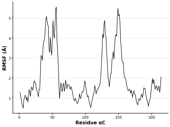
The RMSF is frequently used to determine whether a structure is stable in the simulation’s time-scale. Identifying the higher fluctuations in the 3D protein structure is frequently interesting. MDA allows you to save new trajectories as well as different formats. This allows the user to save the RMSF values as custom B factors and generate a snapshot for visualisation and analysis.
[14]:
u.add_TopologyAttr('tempfactors') #Initialization of B factors (tempfactors) by MDA in the Universe atoms
rmsf=[]
for atom in u.atoms:
    rmsf.append(RMSF_table.loc[atom.resid,'RMSF']) #A new list of RMSF must be created by ATOM. Our table has this values per aC. We can create a longer list easily
[15]:
with mda.Writer("RMSf_factor.pdb", u) as PDB: #This is the functionality from MDA which allos us to save PDB files.
    for ts in u.trajectory[0:1]: #I'll save just the first frame in PDB as snapshot
        u.atoms.tempfactors = rmsf #This adds the custom B factors to the PDB snapshot
        PDB.write(u.atoms)
/mnt/c/Users/angel/Linux_programs/miniconda3/envs/AnalysisMD/lib/python3.7/site-packages/MDAnalysis/coordinates/PDB.py:916: UserWarning: Found no information for attr: 'altLocs' Using default value of ' '
  "".format(attrname, default))
/mnt/c/Users/angel/Linux_programs/miniconda3/envs/AnalysisMD/lib/python3.7/site-packages/MDAnalysis/coordinates/PDB.py:916: UserWarning: Found no information for attr: 'icodes' Using default value of ' '
  "".format(attrname, default))
/mnt/c/Users/angel/Linux_programs/miniconda3/envs/AnalysisMD/lib/python3.7/site-packages/MDAnalysis/coordinates/PDB.py:916: UserWarning: Found no information for attr: 'occupancies' Using default value of '1.0'
  "".format(attrname, default))
/mnt/c/Users/angel/Linux_programs/miniconda3/envs/AnalysisMD/lib/python3.7/site-packages/MDAnalysis/core/topologyattrs.py:1698: VisibleDeprecationWarning: Creating an ndarray from ragged nested sequences (which is a list-or-tuple of lists-or-tuples-or ndarrays with different lengths or shapes) is deprecated. If you meant to do this, you must specify 'dtype=object' when creating the ndarray
  np.array(sorted(unique_bonds)), 4)
After we save the snapshot, the B factor corresponds to our calculated RMSF. The fluctuation can now be seen using py3Dmol, PyMol, or another visualiser.
[21]:
view = py3Dmol.view(js='https://3dmol.org/build/3Dmol.js',height=400,width=600)

view.addModel(open('RMSf_factor.pdb','r').read(),'pdb')

view.setStyle({'cartoon': {'colorscheme': {'prop':'b','gradient': 'roygb','min':min(RMSF_table['RMSF']),'max':max(RMSF_table['RMSF'])}}})

view.show()
You appear to be running in JupyterLab (or JavaScript failed to load for some other reason). You need to install the 3dmol extension:
jupyter labextension install jupyterlab_3dmol
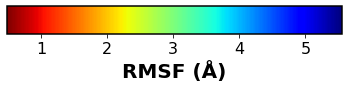
A colorbar to interpret the results
[22]:
fig, ax = plt.subplots(figsize=(6, 1))
fig.subplots_adjust(bottom=0.5)

cmap = mpl.cm.jet_r
norm = mpl.colors.Normalize(vmin=min(RMSF_table['RMSF']), vmax=max(RMSF_table['RMSF']))

cb1 = mpl.colorbar.ColorbarBase(ax, cmap=cmap,norm=norm,orientation='horizontal')
cb1.set_label('RMSF (Å)',fontsize=20,fontweight='bold')
cb1.ax.tick_params(labelsize=16)
fig.show()