Exploring the chemical space by Principal Component Analysis (PCA) and clustering

In this chem-workflow, I will show you how to analyze compound databases in order to identify shared descriptors (physicochemical properties) among them.

A server to perform this analysis (or a similar one) is Platform for Unified Molecular Analysis (PUMA).

For this purpose, I will use a fraction of the REAL Compound Library of Enamine. You can find another example using the same database here.

Importing the libraries we will use

import os
import pandas as pd
import numpy as np
import matplotlib.pyplot as plt
from matplotlib import gridspec

from rdkit import Chem, DataStructs
from rdkit.Chem import Descriptors,Crippen

from sklearn.decomposition import PCA
from sklearn.preprocessing import StandardScaler

import matplotlib.cm as cm
from sklearn.metrics import silhouette_samples, silhouette_score
from sklearn.cluster import KMeans

Loading the molecules

The library contains more than 8 000 000 SMILES codes (size 542.8 M). But we can read the .smiles file as a text file to keep the fist 100 molecules in a pandas table.

# The result of this code will be:
table=pd.DataFrame()
with open('Enamine_REAL_diversity.smiles','r') as file:
    for index,line in enumerate(file):
        if 0<index<=100:
            table.loc[index,'SMILES']=line.split()[0]
            table.loc[index,'Id']=line.split()[1]

Let´s take a look at the first 10 elements of our table of compounds.

table.head(10)

	SMILES	Id
1	CC(C)C(C)(C)SCC=CBr	PV-002312932038
2	CC1CC2(NC(C3CC3C)=NO2)C(C)O1	Z3092470692
3	BrC=CCN1CC2COC(C2)C1	Z3310927277
4	CC(C)CC(C)C(C)NCC1(C)CSC1	Z3362561558
5	CC(C)(C)CS(=O)CC=CCl	Z2904173473
6	CC(C)(C)C1=NOC2(N1)[C@H]1OC[C@H]3C[C@@H]2C[C@@...	Z3092410916
7	BrC=CCNC1CCCC=C1Br	Z3322438014
8	CC(C)C1CC(NCCC2SCCS2)CN1	Z3350500536
9	FCC(CF)NCC1(C(F)F)CC1	PV-002106209714
10	CC(C(F)F)N1N=C(C(F)(F)F)C(F)C1=O	Z2790107381

Molecular descriptors calculation

We can use RDKIT to calculate several molecular descriptors (2D and 3D). However, for this example, we will focus on the descriptors measured in the publication: Platform for Unified Molecular Analysis PUMA 10.1021/acs.jcim.7b00253.

Moreover, a list of all descriptor that can be calculated using RDKIT can be found here.

# We will calculate the descriptors and add them to our table
for i in table.index:
    mol=Chem.MolFromSmiles(table.loc[i,'SMILES'])
    table.loc[i,'MolWt']=Descriptors.ExactMolWt (mol)
    table.loc[i,'TPSA']=Chem.rdMolDescriptors.CalcTPSA(mol) #Topological Polar Surface Area
    table.loc[i,'nRotB']=Descriptors.NumRotatableBonds (mol) #Number of rotable bonds
    table.loc[i,'HBD']=Descriptors.NumHDonors(mol) #Number of H bond donors
    table.loc[i,'HBA']=Descriptors.NumHAcceptors(mol) #Number of H bond acceptors
    table.loc[i,'LogP']=Descriptors.MolLogP(mol) #LogP

As a result, we will get a table with all descriptors for each molecule (SMILES code).

table.head(10)

	SMILES	Id	MolWt	TPSA	nRotB	HBD	HBA	LogP
1	CC(C)C(C)(C)SCC=CBr	PV-002312932038	236.023434	0.00	4.0	0.0	1.0	4.0628
2	CC1CC2(NC(C3CC3C)=NO2)C(C)O1	Z3092470692	210.136828	42.85	1.0	1.0	4.0	1.4693
3	BrC=CCN1CC2COC(C2)C1	Z3310927277	231.025876	12.47	2.0	0.0	2.0	1.6157
4	CC(C)CC(C)C(C)NCC1(C)CSC1	Z3362561558	229.186421	12.03	6.0	1.0	2.0	3.3998
5	CC(C)(C)CS(=O)CC=CCl	Z2904173473	194.053214	17.07	3.0	0.0	1.0	2.5337
6	CC(C)(C)C1=NOC2(N1)[C@H]1OC[C@H]3C[C@@H]2C[C@@...	Z3092410916	236.152478	42.85	0.0	1.0	4.0	1.7169
7	BrC=CCNC1CCCC=C1Br	Z3322438014	292.941474	12.03	3.0	1.0	1.0	3.3159
8	CC(C)C1CC(NCCC2SCCS2)CN1	Z3350500536	260.138091	24.06	5.0	2.0	4.0	2.1587
9	FCC(CF)NCC1(C(F)F)CC1	PV-002106209714	199.098412	12.03	6.0	1.0	1.0	1.9289
10	CC(C(F)F)N1N=C(C(F)(F)F)C(F)C1=O	Z2790107381	248.038432	32.67	2.0	0.0	2.0	1.7386

Principal Component Analysis of calculated molecular descriptors (PCA)

I won´t discuss the basis of PCA due to this site is focused on workflows. However, PCA analysis for different application has been discussed plenty. As a quick reference, you can visit the PCA explanation at Wikipedia.

For our analysis, we need to select the values of the table that we will use for PCA. Meaning, the descriptors we calculated.

descriptors = table.loc[:, ['MolWt', 'TPSA', 'nRotB', 'HBD','HBA', 'LogP']].values

A very important step is performing a standardization of the scales of the descriptors. Scales differences in PCA modify the variance distribution during PCA. More info about this topic can be found here.

descriptors_std = StandardScaler().fit_transform(descriptors)

Now, we are ready to calculate the PCA

pca = PCA()
descriptors_2d = pca.fit_transform(descriptors_std)

Let´s add the PCA data to a new table

descriptors_pca= pd.DataFrame(descriptors_2d)
descriptors_pca.index = table.index
descriptors_pca.columns = ['PC{}'.format(i+1) for i in descriptors_pca.columns]
descriptors_pca.head(10)

	PC1	PC2	PC3	PC4	PC5	PC6
1	-2.463784	-0.936078	-0.274030	0.558761	-0.063431	0.131835
2	-0.075200	1.908703	-0.534952	0.042434	-0.559363	-0.252494
3	-1.477081	0.865532	-1.070530	-0.451302	0.453224	-0.201938
4	-1.526756	-0.336039	1.094536	0.286876	-0.170061	-0.175008
5	-2.147808	0.475692	-0.564722	-0.344079	-0.139551	0.425832
6	0.066967	1.802380	-0.849193	0.543555	-0.370788	-0.232141
7	-1.384515	-0.041261	0.202822	1.299544	0.823427	0.123817
8	0.083638	0.888434	1.430529	0.522356	0.088537	-0.931776
9	-1.817628	0.741035	1.132660	-0.646553	0.332754	-0.019503
10	-0.899886	0.776893	-1.091563	-0.339891	0.401541	0.382843

We can check the explained variance to see the variance explained by each component from PCA

print(pca.explained_variance_ratio_)
print(sum(pca.explained_variance_ratio_))

[0.42278681 0.30201227 0.14303101 0.08478587 0.03041105 0.01697299]
1.0

And also, we can plot such data

plt.rcParams['axes.linewidth'] = 1.5
plt.figure(figsize=(8,6))
fig, ax = plt.subplots(figsize=(8,6))

var=np.cumsum(np.round(pca.explained_variance_ratio_, decimals=3)*100)
plt.plot([i+1 for i in range(len(var))],var,'k-',linewidth=2)
plt.xticks([i+1 for i in range(len(var))])
plt.ylabel('% Variance Explained',fontsize=16,fontweight='bold')
plt.xlabel('Pincipal Component (PC)',fontsize=16,fontweight='bold')
ax.spines['top'].set_visible(False)
ax.spines['right'].set_visible(False)
plt.tight_layout()
plt.tick_params ('both',width=2,labelsize=12)

<Figure size 576x432 with 0 Axes>

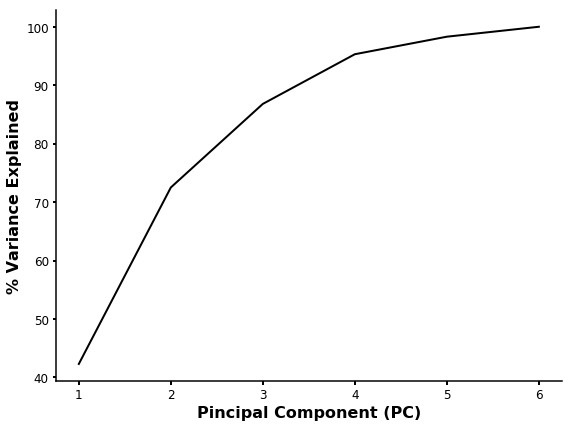
As you can see, the PC1 and PC2 explain 72.4 % of the variability. So we can plot PC1 vs PC2 to see the distribution of our compounds.

fig = plt.figure(figsize=(8,6))
ax = fig.add_subplot(111)

ax.plot(descriptors_pca['PC1'],descriptors_pca['PC2'],'o',color='k')
ax.set_title ('Principal Component Analysis',fontsize=16,fontweight='bold',family='sans-serif')
ax.set_xlabel ('PC1',fontsize=14,fontweight='bold')
ax.set_ylabel ('PC2',fontsize=14,fontweight='bold')

plt.tick_params ('both',width=2,labelsize=12)

plt.tight_layout()
plt.show()

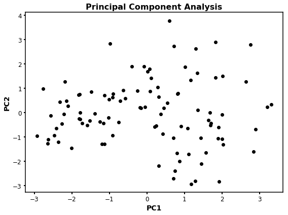
However, this plot is simple and we cannot identify compound clusters easily. For such purpose, we can perform clustering analysis using the PCA values to identify compound groups by mathematical approaches. Moreover, PC1 vs PC2 (or any other combination) won´t give us information about which feature (descriptor) is more important to explain the variance of our values.

For this example, we will identify the most important feature (descriptor), and we identify compound clusters by the k-means clustering algorithm. For more info about k-means, you can look at skit-learn.

K-means clustering and main features identification

The first step for this analysis is to re-scale our PCA values from -1 to 1. This because we want to analyze our data inside of the covariance cycle of the features (descriptors). Fur such purpose we type:

# This normalization will be performed just for PC1 and PC2, but can be done for all the components.
scale1 = 1.0/(max(descriptors_pca['PC1']) - min(descriptors_pca['PC1']))
scale2 = 1.0/(max(descriptors_pca['PC2']) - min(descriptors_pca['PC2']))

# And we add the new values to our PCA table
descriptors_pca['PC1_normalized']=[i*scale1 for i in descriptors_pca['PC1']]
descriptors_pca['PC2_normalized']=[i*scale2 for i in descriptors_pca['PC2']]

descriptors_pca.head(10)

	PC1	PC2	PC3	PC4	PC5	PC6	PC1_normalized	PC2_normalized
1	-2.463784	-0.936078	-0.274030	0.558761	-0.063431	0.131835	-0.395072	-0.139342
2	-0.075200	1.908703	-0.534952	0.042434	-0.559363	-0.252494	-0.012058	0.284125
3	-1.477081	0.865532	-1.070530	-0.451302	0.453224	-0.201938	-0.236852	0.128841
4	-1.526756	-0.336039	1.094536	0.286876	-0.170061	-0.175008	-0.244818	-0.050022
5	-2.147808	0.475692	-0.564722	-0.344079	-0.139551	0.425832	-0.344405	0.070810
6	0.066967	1.802380	-0.849193	0.543555	-0.370788	-0.232141	0.010738	0.268298
7	-1.384515	-0.041261	0.202822	1.299544	0.823427	0.123817	-0.222009	-0.006142
8	0.083638	0.888434	1.430529	0.522356	0.088537	-0.931776	0.013412	0.132250
9	-1.817628	0.741035	1.132660	-0.646553	0.332754	-0.019503	-0.291460	0.110309
10	-0.899886	0.776893	-1.091563	-0.339891	0.401541	0.382843	-0.144298	0.115646

fig = plt.figure(figsize=(8,6))
ax = fig.add_subplot(111)

ax.plot(descriptors_pca['PC1_normalized'],descriptors_pca['PC2_normalized'],'o',color='k')
ax.set_title ('Principal Component Analysis',fontsize=16,fontweight='bold',family='sans-serif')
ax.set_xlabel ('PC1',fontsize=14,fontweight='bold')
ax.set_ylabel ('PC2',fontsize=14,fontweight='bold')

plt.tick_params ('both',width=2,labelsize=12)

plt.tight_layout()
plt.show()

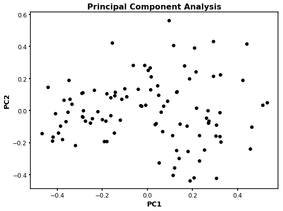
As you can see, the distribution of the points is the same as before, however, the scale now is from -1 to 1.

k-means clustering

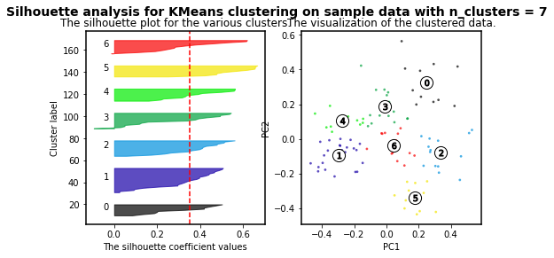
K-means clustering is an algorithm in which the user must define the number of clusters. However, in order to mathematically select a number of clusters for a group of points based on distribution, different algorithms can be applied. For instance, we will use the silhouette-based algorithm to identify the best number of clusters for our distribution. More info about silhouette algorithm can be found here and here.

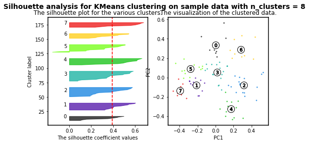
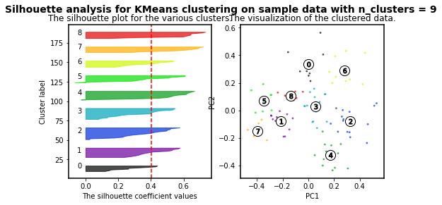
range_n_clusters = [2, 3, 4, 5, 6, 7,8,9,10]
for n_clusters in range_n_clusters:
    fig, (ax1,ax2)= plt.subplots(1, 2)
    fig.set_size_inches(8, 4)

    kmeans = KMeans(n_clusters=n_clusters, random_state=10)
    cluster_labels = kmeans.fit_predict(descriptors_pca[['PC1_normalized','PC2_normalized']])
    silhouette_avg = silhouette_score(descriptors_pca[['PC1_normalized','PC2_normalized']], cluster_labels)
    print("For n_clusters =", n_clusters,
          "The average silhouette_score is :", silhouette_avg)

    sample_silhouette_values = silhouette_samples(descriptors_pca[['PC1_normalized','PC2_normalized']], cluster_labels)

    y_lower = 10

    for i in range(n_clusters):
        # Aggregate the silhouette scores for samples belonging to
        # cluster i, and sort them
        ith_cluster_silhouette_values = \
            sample_silhouette_values[cluster_labels == i]

        ith_cluster_silhouette_values.sort()

        size_cluster_i = ith_cluster_silhouette_values.shape[0]
        y_upper = y_lower + size_cluster_i

        color = cm.nipy_spectral(float(i) / n_clusters)
        ax1.fill_betweenx(np.arange(y_lower, y_upper),
                          0, ith_cluster_silhouette_values,
                          facecolor=color, edgecolor=color, alpha=0.7)

        # Label the silhouette plots with their cluster numbers at the middle
        ax1.text(-0.05, y_lower + 0.5 * size_cluster_i, str(i))

        # Compute the new y_lower for next plot
        y_lower = y_upper + 10  # 10 for the 0 samples

    ax1.set_title("The silhouette plot for the various clusters.")
    ax1.set_xlabel("The silhouette coefficient values")
    ax1.set_ylabel("Cluster label")

    # The vertical line for average silhouette score of all the values
    ax1.axvline(x=silhouette_avg, color="red", linestyle="--")


    # 2nd Plot showing the actual clusters formed
    colors = cm.nipy_spectral(cluster_labels.astype(float) / n_clusters)
    ax2.scatter(descriptors_pca['PC1_normalized'], descriptors_pca['PC2_normalized'],
                marker='.', s=30, lw=0, alpha=0.7,c=colors, edgecolor='k')


    # Labeling the clusters
    centers = kmeans.cluster_centers_
    # Draw white circles at cluster centers
    ax2.scatter(centers[:, 0], centers[:, 1], marker='o',
                c="white", alpha=1, s=200, edgecolor='k')

    for i, c in enumerate(centers):
        ax2.scatter(c[0], c[1], marker='$%d$' % i, alpha=1,
                    s=50, edgecolor='k')

    ax2.set_title("The visualization of the clustered data.")
    ax2.set_xlabel("PC1")
    ax2.set_ylabel("PC2")

    plt.suptitle(("Silhouette analysis for KMeans clustering on sample data "
                  "with n_clusters = %d" % n_clusters),
                 fontsize=14, fontweight='bold')


plt.show()

For n_clusters = 2 The average silhouette_score is : 0.4084228227138712
For n_clusters = 3 The average silhouette_score is : 0.45489833249431
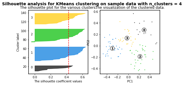
For n_clusters = 4 The average silhouette_score is : 0.4241945808059022
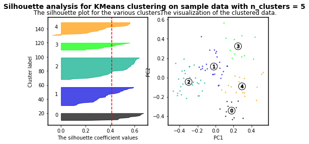
For n_clusters = 5 The average silhouette_score is : 0.4131292685513735
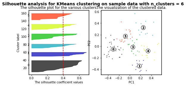
For n_clusters = 6 The average silhouette_score is : 0.39907782063536723
For n_clusters = 7 The average silhouette_score is : 0.3523945319600729
For n_clusters = 8 The average silhouette_score is : 0.3906505698840795
For n_clusters = 9 The average silhouette_score is : 0.4003463850492715
For n_clusters = 10 The average silhouette_score is : 0.384264972688578

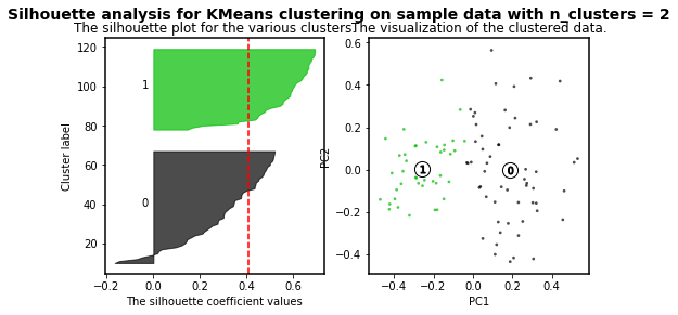
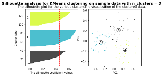
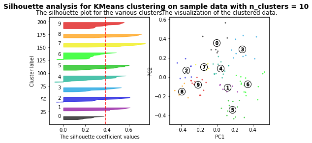
As higher the silhouette_score the better cluster distribution. Then, for our data:

For n_clusters = 3 The average silhouette_score is : 0.45489833249431

3 clusters are the best for our data distribution. So, let´s use such number of clusters.

kmeans = KMeans(n_clusters=3, random_state=10) # We define the best number of clusters
clusters = kmeans.fit(descriptors_pca[['PC1_normalized','PC2_normalized']]) #PC1 vs PC2 (normalized values)

Once the calculation of clusters is done, we can add the result to our PCA table.

descriptors_pca['Cluster_PC1_PC2'] = pd.Series(clusters.labels_, index=table.index)

descriptors_pca.head(10)

	PC1	PC2	PC3	PC4	PC5	PC6	PC1_normalized	PC2_normalized	Cluster_PC1_PC2
1	-2.463784	-0.936078	-0.274030	0.558761	-0.063431	0.131835	-0.395072	-0.139342	1
2	-0.075200	1.908703	-0.534952	0.042434	-0.559363	-0.252494	-0.012058	0.284125	0
3	-1.477081	0.865532	-1.070530	-0.451302	0.453224	-0.201938	-0.236852	0.128841	1
4	-1.526756	-0.336039	1.094536	0.286876	-0.170061	-0.175008	-0.244818	-0.050022	1
5	-2.147808	0.475692	-0.564722	-0.344079	-0.139551	0.425832	-0.344405	0.070810	1
6	0.066967	1.802380	-0.849193	0.543555	-0.370788	-0.232141	0.010738	0.268298	0
7	-1.384515	-0.041261	0.202822	1.299544	0.823427	0.123817	-0.222009	-0.006142	1
8	0.083638	0.888434	1.430529	0.522356	0.088537	-0.931776	0.013412	0.132250	0
9	-1.817628	0.741035	1.132660	-0.646553	0.332754	-0.019503	-0.291460	0.110309	1
10	-0.899886	0.776893	-1.091563	-0.339891	0.401541	0.382843	-0.144298	0.115646	1

Now everything together

We will plot PC1 vs PC2 data. Each cluster will have a different color, and we will find the main feature for each principal component.

plt.rcParams['axes.linewidth'] = 1.5
plt.figure(figsize=(10,8))

fig, ax = plt.subplots(figsize=(7,7))

color_code={ 0:        'magenta',\
             1.0:   'orange',\
             2.0:      'cyan',\
             3.0:           'c',\
             4.0:        'm',\
             5.0:        'y',\
             6.0:        'darkorange',
             7.0:       'k',
             }

for i in descriptors_pca.index:
        ax.plot(descriptors_pca.loc[i].at['PC1_normalized'],descriptors_pca.loc[i].at['PC2_normalized'],
                    c=color_code[descriptors_pca.loc[i].at['Cluster_PC1_PC2']],
                    marker='o',markersize=8,markeredgecolor='k',alpha=0.3)


plt.xlabel ('PC1',fontsize=14,fontweight='bold')
ax.xaxis.set_label_coords(0.98, 0.45)
plt.ylabel ('PC2',fontsize=14,fontweight='bold')
ax.yaxis.set_label_coords(0.45, 0.98)
plt.tick_params ('both',width=2,labelsize=12)
ax.spines['left'].set_position(('data', 0))
ax.spines['bottom'].set_position(('data', 0))
ax.spines['top'].set_visible(False)
ax.spines['right'].set_visible(False)

lab=['MolWt', 'TPSA', 'nRotB', 'HBD','HBA', 'LogP'] #Feature labels

l=np.transpose(pca.components_[0:2, :]) ## We will get the components eigenvectors (main features) for PC1 and PC2

n = l.shape[0]
for i in range(n):
    plt.arrow(0, 0, l[i,0], l[i,1],color= 'k',alpha=0.6,linewidth=1.2,head_width=0.025)
    plt.text(l[i,0]*1.25, l[i,1]*1.25, lab[i], color = 'k',va = 'center', ha = 'center',fontsize=11)

circle = plt.Circle((0,0), 1, color='gray', fill=False,clip_on=True,linewidth=1.5,linestyle='--')
ax.add_artist(circle)
plt.xlim(-1.2,1.2)
plt.ylim(-1.2,1.2)
plt.tight_layout()
plt.show()

<Figure size 720x576 with 0 Axes>

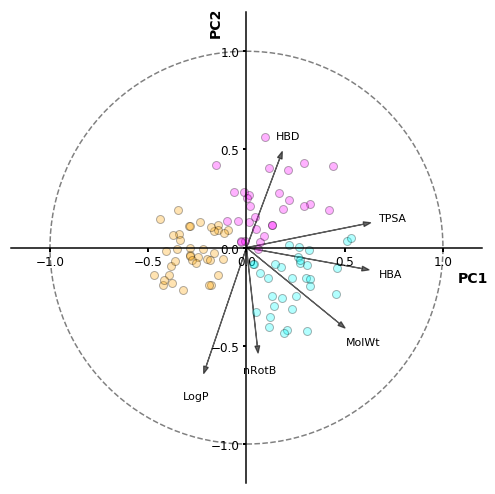
As a result, we can identify the features that correlate positively and negatively with PC1 (TPSA, HBA, MolWt), and with PC2 (HBD, nRotB, LogP). Additionally, we can see that LogP is the “most important” feature (descriptor) because of the vector length. And also we can see the 3 different clusters we identified by the silhouette-based algorithm.

Finally, we can merge our tables to keep the data in a single table or file.

table=table.join(descriptors_pca)

table.head(10)

	SMILES	Id	MolWt	TPSA	nRotB	HBD	HBA	LogP	PC1	PC2	PC3	PC4	PC5	PC6	PC1_normalized	PC2_normalized	Cluster_PC1_PC2
1	CC(C)C(C)(C)SCC=CBr	PV-002312932038	236.023434	0.00	4.0	0.0	1.0	4.0628	-2.463784	-0.936078	-0.274030	0.558761	-0.063431	0.131835	-0.395072	-0.139342	1
2	CC1CC2(NC(C3CC3C)=NO2)C(C)O1	Z3092470692	210.136828	42.85	1.0	1.0	4.0	1.4693	-0.075200	1.908703	-0.534952	0.042434	-0.559363	-0.252494	-0.012058	0.284125	0
3	BrC=CCN1CC2COC(C2)C1	Z3310927277	231.025876	12.47	2.0	0.0	2.0	1.6157	-1.477081	0.865532	-1.070530	-0.451302	0.453224	-0.201938	-0.236852	0.128841	1
4	CC(C)CC(C)C(C)NCC1(C)CSC1	Z3362561558	229.186421	12.03	6.0	1.0	2.0	3.3998	-1.526756	-0.336039	1.094536	0.286876	-0.170061	-0.175008	-0.244818	-0.050022	1
5	CC(C)(C)CS(=O)CC=CCl	Z2904173473	194.053214	17.07	3.0	0.0	1.0	2.5337	-2.147808	0.475692	-0.564722	-0.344079	-0.139551	0.425832	-0.344405	0.070810	1
6	CC(C)(C)C1=NOC2(N1)[C@H]1OC[C@H]3C[C@@H]2C[C@@...	Z3092410916	236.152478	42.85	0.0	1.0	4.0	1.7169	0.066967	1.802380	-0.849193	0.543555	-0.370788	-0.232141	0.010738	0.268298	0
7	BrC=CCNC1CCCC=C1Br	Z3322438014	292.941474	12.03	3.0	1.0	1.0	3.3159	-1.384515	-0.041261	0.202822	1.299544	0.823427	0.123817	-0.222009	-0.006142	1
8	CC(C)C1CC(NCCC2SCCS2)CN1	Z3350500536	260.138091	24.06	5.0	2.0	4.0	2.1587	0.083638	0.888434	1.430529	0.522356	0.088537	-0.931776	0.013412	0.132250	0
9	FCC(CF)NCC1(C(F)F)CC1	PV-002106209714	199.098412	12.03	6.0	1.0	1.0	1.9289	-1.817628	0.741035	1.132660	-0.646553	0.332754	-0.019503	-0.291460	0.110309	1
10	CC(C(F)F)N1N=C(C(F)(F)F)C(F)C1=O	Z2790107381	248.038432	32.67	2.0	0.0	2.0	1.7386	-0.899886	0.776893	-1.091563	-0.339891	0.401541	0.382843	-0.144298	0.115646	1

Saving values from a pandas table to a .csv file is very easy. You just need to type:

table.to_csv('file_name.csv')